In mathematics, a geodesic is a generalization of the notion of a "straight line" to "curved spaces". In presence of a metric, geodesics are defined to be (locally) the shortest path between points on the space. In the presence of an affine connection, geodesics are defined to be curves whose tangent vectors remain parallel if they are transported along it.
The term "geodesic" comes from geodesy, the science of measuring the size and shape of Earth; in the original sense, a geodesic was the shortest route between two points on the Earth's surface, namely, a segment of a great circle. The term has been generalized to include measurements in much more general mathematical spaces; for example, in graph theory, one might consider a geodesic between two vertices/nodes of a graph.
Geodesics are of particular importance in general relativity.
Examples
In metric geometry, a geodesic is a curve which is everywhere locally a distance minimizer. More precisely, a curve γ: I → M from the unit interval I to the metric space M is a geodesic if there is a constant v ≥ 0 such that for any t ∈ I there is a neighborhood J of t in I such that for any t1, t2 ∈ J we have

This generalizes the notion of geodesic for Riemannian manifolds. However, in metric geometry the geodesic considered is almost always equipped with natural parametrization, i.e. in the above identity v = 1 and

If the last equality is satisfied for all t1, t2 ∈I, the geodesic is called a minimizing geodesic or shortest path.
In general, a metric space may have no geodesics, except constant curves.
Metric geometry
Just as in a standard metric space, a geodesic on a (pseudo-)Riemannian manifold M is defined as a curve γ(t) minimizes the length of the curve. Explicitly, we can write the length of any curve as

where
 represents the derivative with respect to t, and is a vector. The sign in the square root is chosen once for a given curve, to ensure that the square root is a real number. The positive sign is chosen for spacelike curves; in a pseudo-Riemannian manifold, the negative sign may be chosen for timelike curves. A geodesic, then, is the curve which extremizes this quantity (locally).
In the case of a manifold with torsion-free and metric-compatible connection (which is almost always assumed to be the case in Relativity, for example), a geodesic curve is also an autoparallel curve. That is, the curve parallel transports its own tangent vector, so

at each point along the curve. Here, ∇ stands for the Levi-Civita connection on M.
In this case, using local coordinates on M, we can write the geodesic equation (using the summation convention) as
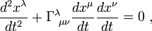
where x(t) are the coordinates of the curve γ(t) and
 are the Christoffel symbols. This is just an ordinary differential equation for the coordinates. It has a unique solution, given an initial position and an initial velocity. Therefore, from the point of view of classical mechanics, geodesics can be thought of as trajectories of free particles in a manifold.
Geodesics can also be defined as extremal curves for the following action functional

where g is a Riemannian (or pseudo-Riemannian) metric. In pure mathematics, this quantity would generally be referred to as an energy. The geodesic equation can then be obtained as the Euler-Lagrange equations of motion for this action.
In a similar manner, one can obtain geodesics as a solution of the Hamilton–Jacobi equations, with (pseudo-)Riemannian metric taken as Hamiltonian. See Riemannian manifolds in Hamiltonian mechanics for further details.
 (Pseudo-)Riemannian geometry
The local existence and uniqueness theorem for geodesics states that geodesics exist, and are unique; this is a variant of the Frobenius theorem. More precisely:
For any point p in M and for any vector V in TpM (the tangent space to M at p) there exists a unique geodesic
 : I → M such that
 and
and
 ,
,
where I is a maximal open interval in R containing 0.
In general, I may not be all of R as for example for an open disc in R². The proof of this theorem follows from the theory of ordinary differential equations, by noticing that the geodesic equation is a second-order ODE. Existence and uniqueness then follow from the Picard-Lindelöf theorem for the solutions of ODEs with prescribed initial conditions. γ depends smoothly on both p and V.
Existence and uniqueness
Geodesic flow is an -action on tangent bundle T(M) of a manifold M defined in the following way

where ,
,  and γV denotes the geodesic with initial data
  .
.
It defines a Hamiltonian flow on (co)tangent bundle with the (pseudo-)Riemannian metric as the Hamiltonian. In particular it preserves the (pseudo-)Riemannian metric g, i.e.
g(G(V)) = g(V,V).
That makes possible to define geodesic flow on unit tangent bundle UT(M) of the Riemannian manifold M.
 Geodesic flow
The geodesic flow defines a family of curves in the tangent bundle. The derivatives of these curves define a vector field on the total space of the tangent bundle, known as the geodesic spray.
Affine and projective geodesics
Basic introduction to the mathematics of curved spacetime
Complex geodesic
Differential geometry of curves
Exponential map
Geodesic dome
Geodesic (general relativity)
Geodesics as Hamiltonian flows
Hopf-Rinow theorem
Intrinsic metric
Jacobi field
Quasigeodesic
Solving the geodesic equations
Barnes Wallis, who applied geodesics to aircraft structural design in the design of the Vickers Wellesley and Vickers Wellington aircraft, and the R100 airship.
 Lefthit