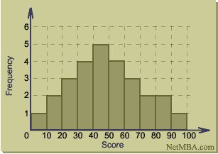
In statistics, a histogram is a graphical display of tabulated frequencies. A histogram is the graphical version of a table that shows what proportion of cases fall into each of several or many specified categories. The histogram differs from a bar chart in that it is the area of the bar that denotes the value, not the height, a crucial distinction when the categories are not of uniform width (Lancaster, 1974). The categories are usually specified as non-overlapping intervals of some variable. The categories (bars) must be adjacent.
The word histogram is derived from Greek: histos 'anything set upright' (as the masts of a ship, the bar of a loom, or the vertical bars of a histogram); gramma 'drawing, record, writing'. The histogram is one of the seven basic tools of quality control, which also include the Pareto chart, check sheet, control chart, cause-and-effect diagram, flowchart, and scatter diagram. A generalization of the histogram is kernel smoothing techniques. This will construct a very smooth Probability density function from the supplied data.
Examples
The SOCR resource pages contain a number of hands-on interactive activities demonstrating the concept of a Histogram, histogram construction and manipulation using Java applets and charts.
Activities and demonstrations
In a more general mathematical sense, a histogram is simply a mapping mi that counts the number of observations that fall into various disjoint categories (known as bins), whereas the graph of a histogram is merely one way to represent a histogram. Thus, if we let n be the total number of observations and k be the total number of bins, the histogram mi meets the following conditions:

 Mathematical definition
A cumulative histogram is a mapping that counts the cumulative number of observations in all of the bins up to the specified bin. That is, the cumulative histogram Mi of a histogram mi is defined as:

Cumulative Histogram
There is no "best" number of bins, and different bin sizes can reveal different features of the data. Some theoreticians have attempted to determine an optimal number of bins, but these methods generally make strong assumptions about the shape of the distribution. You should always experiment with bin widths before choosing one (or more) that illustrate the salient features in your data.
The number of bins k can be calculated directly, or from a suggested bin width h:

The braces indicate the ceiling function.

which implicitly bases the bin sizes on the range of the data, and can perform poorly if n < 30.

where h is the common bin width, and s is the sample standard deviation.

which is based on the interquartile range
 Lefthit